Analysis of Quantitative Data

Chapter 12

Introduction

This chapter provides information about the analysis of quantitative data based on the assumption that the data has already been collected (as described in previous chapters.)  Quantitative research emphasizes the precise measurement of variables and testing of hypotheses that are linked to general causal explanations (pg. 122). The primary aim of quantitative research is to determine what relationship exists between an independent variable and a dependent variable.  Researchers do several things to the raw data, to provide meaning. This type of data is usually expressed using charts, graphs and numbers. The research can be descriptive where subjects are measured once and a relationship between them is identified.  It can also be experiential where subjects are measured prior to and after some form of treatment.  From the data, causalities are identified.  

http://people.biola.edu/faculty/richs/ed/Chapter4/Chap4Index.htm

http://www.sportsci.org/jour/0001/wghdesign.html

Dealing With Data

A. Coding Data  

This is the systematic reorganization of raw data into a format that is machine-readable. This must be completed before testing hypotheses. When coding data researchers use a coding procedure, “which is a set of rules stating that certain numbers are assigned to variable attributes” (pg. 341).   Making a backup copy of your codebook is highly recommended in case the original is destroyed.  The codebook is the key to your coded data.  The challenge can be coding answers for open-ended survey questions.

http://www.nova.edu/ssss/QR/QR3-1/carney.html

B. Entering Data  

Data analysis using computer programs will usually utilize a grid format.  Researchers translate raw data into computer format using; code sheets, direct entry, optical scan sheets, or computer-assisted telephone interviewing. Data analysis using computer programs will usually utilize a grid format similar to that found in software packages such as Microsoft Excel or WordPerfect

http://www.rti.org/units/shsp/factsheets/B007.cfm

http://www.uncg.edu/tlc/opscan2.htm

C. Cleaning Data

Accurately coding data is of extreme importance as errors in coding can ruin or invalidate results.  A few different tests can be run to verify data and identify data errors.  These include wild code random code checking and logically cross checking two or more variables.    

Results With One Variable

A. Frequency Distributions

The chapter describes two types of statistics but focuses on ways to manipulate and summarize numbers that represent data from a research project.  Frequency distribution is illustrated as a method of describing numerical data of one variable.  Graphic methods of displaying the data include pie charts, bar charts, and histograms.    

http://www.psychstat.smsu.edu/introbook/sbk07.htm

B. Measures of Central Tendency  

This is a procedure used to summarize the information regarding one variable into a single number.  We commonly see this expressed in three forms:  

1. The mode, (eyeball) is the most frequently occurring number in a set.
2. The median is the middle number (50^th percentile) in a set.
3. The mean is the average of the numbers in a set.

If the results formed from the frequency distribution form a normal bell curve, the values of the above three mentioned terms tend to be very close to one another or are equal.  If the distribution is skewed, then the three will not be equal .

http://davidmlane.com/hyperstat/A39322.html

C. Measures of Variation

Variation is the spread, dispersion, or variability around the center of the set.  This is an important aspect of researchers because if the variation of data is unknown, data could very well be misinterpreted.   Zero variation means that every value in the set is equal to the mean and median.   The range involves the difference between the largest and smallest scores in that set of data.  To describe a specific place in the distribution, a percentile can be used.  For example, the median is the 50^th percentile.  Standard deviation is the most commonly used measure of variation.  Along with the mean, it is used to calculate z-scores, which act like a standardized score.  A researcher can use a z-score to compare multiple groups of data.

Standard Deviation

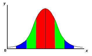
Standard deviation is a mathematical measure of variability that can give us a relative measure of the amount to which each score in a set of data differs from the mean of that data.  The following is a brief explanation regarding a normal distribution and standard deviation and z-scores.

  When dealing with a normal distribution of data (normal symmetrical bell curve with the mean in the center) from score results, 34% of scores will fall one (1) standard deviation below the mean and 34% will fall one (1) standard deviation above the mean.  In total 68% of all scores should fall within one (1) +/- standard deviation from the mean.  Another 14% will fall between one (1) and two (2) +/- standard deviations from the mean.  The remaining 4% of scores will fall greater than two (2) +/- standard deviations away from the mean. 

  Please see Figure 1 below for graphical display.

                          -2s    -1s     mean    +1s     +2s

Figure 1: Normal Distribution Curve Indicating Areas Associated with Standard Deviation

For example, You have a normal distribution of scores and the mean is calculated to be 75 and the standard deviation to be 5.  68% of scores will be in the 70 – 80 range which is one standard deviation (+/-) from the mean.  If a student scores 65, they are two standard deviations (-) away from the mean.

Z-Scores

A z-score tells us how many standard deviations exist between a score and the mean.  Z-scores may either be positive or negative (+/-).  A positive z-score tells us the score is above the mean and a negative z-score indicates a score lower than the mean.  If a subject has a z-score of +1 then they lie +1 standard deviation of the mean.

Z-scores can also tell us where scores stand in relation to other scores in the same test and on other tests. 

Suppose:

Science Test                                                         Math Test            

mean = 75                                                              mean = 80

standard deviation = 5                                        standard deviation = 7

Results With Two Variables

A. Bivariate Relationships

Bivariate relationships show a statistical relationship between variables through the consideration of two variables together and their corresponding relationships.  Variables may relate through covariation which means that they are associated or do affect each other.  On the other hand, independent variables have no association and no affect on one another.  Independence opposes covariation.  Evidence supporting a null hypothesis indicates independence.  Covariance is often exemplified when there is evidence supporting a straight-forward hypothesis.  Three techniques are often used to help express whether a relationship exists or not between variables:

1.      Scattergrams, graph, or plot of the relationship

2.      Cross-tabulation or a percentage table

3.      Measures of association - statistical measures that express the amount of covariation by a single number called a correlation coefficient

http://disc-nt.cba.uh.edu/chin/surv.html

B. Assessing Survey Research

    I. The Scattergram

“A scattergram is a graph on which a researcher plots each case or observation, where each axis represents the value of one variable.” (pg. 323)  Researchers can gain valuable information through the use of scattergrams.  The form, direction and precision related to the relationship between variables reveal critical details about research data. Three types of possible relationship may be observed:

1. Curvilinear relationship
2. Linear
3. Independent

1	500
2	1000
3	1200
4	1500
5	2500
6	5000
7	5500
8	7000
9	8000
10	10000
11	15000
12	22000
13	30000
14	40000
15	50000
1	100
2	90
3	80
4	70
5	60
6	50
7	40
8	30
9	20
10	10
2	100
4	7
6	12
8	200
10	160
12	65
14	70
16	10
18	150
20	88

http://davidmlane.com/hyperstat/desc_biv.html

    II. Bivariate Tables

Bivariate tables present the same information as a scattergram but is more condensed and based on cross-tabulation.  Here, cases are organized on the basis of two variables at the same time.   A percentage table is a form of bivariate table.  If there is no relationship present in the table the percentage values will look equal across the columns or rows.  Large percentages in the diagonal rows indicate a linear relationship.  Large patterns across cells may indicate a curvilinear relationship between variables.  Please see example of table on page 328, Neuman.  The principles of reading a scattergram can help you see a relationship in a percentage table.  A positive relationship indicates that one variable increases with the other.  A negative relationship indicates that one variable increases as the other decreases.

http://axe.acadiau.ca/~040662t/collapsedbivariatepercentage.htm

http://axe.acadiau.ca/~040662t/percentagetables.htm

    III. Measures of Association

“A measure of association is a single number that expresses the strength, and often the direction, of a relationship.  It condenses information about a bivariate relationship into a single number” (pg. 330).   When determining the correlation one needs to determine a correlation coefficient; if the variables are independent the correlation coefficient is equal to zero. Values in the range of 0 to –1 indicate a negative correlation with –1 being the strongest.  Values in the range from 0 to +1 indicate a positive correlation with +1 being the strongest.  There are five measures of association represented by the Greek symbols Lambda, Gamma, Tau, Rho, and Chi-square.

  http://www.tgc.com/dsstar/99/1116/101141.html

More Than Two Variables

A. Statistical Control

Researchers eliminate alternative explanations of variable relationships by using statistical control. Caution is exercised in interpreting these relationships until control variables have been considered.  This is done by selecting a research design that allows for control of other potential explanations by including a third variable and determining what affect it has on the relationship.  If it has no effect, the bivariate relationship is not considered spurious.

  http://akao.larc.nasa.gov/dfc/sqc.html

 B. The Elaboration Model of Percentaged Tables

To eliminate spuriousness researchers determine whether alternative explanations better describe relationships than that of the causal relationship.  A trivariate table has a bivariate table of the independent and dependent for each category of the control variable.  Using the data, a table containing partials can be formed with the number of partials determined by the number of categories in the control variable.  Trivariate tables can be difficult to interpret, certain types of control variables must be grouped and the outcomes can be affected by the groupings chosen.

 http://carbon.cudenver.edu/~bwilson/elab.html

 C.  Multiple Regression Analysis

Multiple regression analysis assists in the reduction of error in data analysis and is usually administered using a statistical computer program due to the complexity of the computation.  This data tells us how well a variable explains a dependent variable and the direction and size of that effect.  This statistical technique requires interval or ratio-level data and tells the reader how well a set of variables explains dependent variables.  Regressions results measure the direction and size of the effect and is measured precisely and given a numerical value.

 http://www.statsoftinc.com/textbook/stmulreg.html#cthe

http://www.windsor.igs.net/~nhodgins/multiple_regression_research_analysis.html

  Inferential Statistics

 A. The Purpose of Inferential Statistics

 Inferential statistics are used by researchers in an attempt to express their confidence when transferring experimental results to that of the greater population and indicate the probability of finding the results in the population.  Researchers use probability theory to test hypotheses formally, permit inferences from a sample population, and test whether descriptive results are likely due to random factors or to a real relationship (pg 338).

 These statistics are useful but limited as the data must come from a random sample and thus sampling errors must be taken into account.  This does some to eliminate error however, non-sampling errors are not considered. 

  http://www.ruf.rice.edu/~lane/hyperstat/A29136.html

B. Statistical Significance

Statistical significance determines that the results are not due to chance factors but cannot prove absolute certainty as it only reports if results are produced by random error.  It states the probability of finding a relationship in the sample, when there isn’t one in the population. Results can be theoretically meaningless as it is a random process and the sample results will differ within population parameters

 http://www.surveysystem.com/signif.htm

C. Levels of Significance

 Levels of significance are based on probability theory linking sample data to a population.  It describes the statistical significance in terms of the specific probability thus allowing researchers the opportunity to state their confidence in the probability.  A 0.95 or 95% level of significance usually is an accepted level.  0.05 or 5% is left open for chance or random error.

 http://www.salford.ac.uk/healthSci/resmeth2000/resmeth/signific.htm

D. Type I and Type II Errors

 “A Type 1 error occurs when the researcher says that a relationship exists when in fact none exists.  It means falsely rejecting a null hypothesis.  A Type II error occurs when a researcher says that a relationship does not exist when in fact it does” (pg. 339).

 http://www.ruf.rice.edu/~lane/hyperstat/A18652.html

Conclusion  

“Goal of scientific research is to produce knowledge that truly reflects the social world, not to defend pet ideas or hypotheses.” (page 342)

Quantitative analysis and interpretation of the results can be difficult and confusing.  Good quantitative results are highly dependent on sound methodology.  It is important to not try to set yourself into looking for results that will only support your initial hypothesis.  Many new hypothesis and ideas can result from the final outcomes. 

 One must be wary that quantitative data and statistics are not misused in an attempt to sway or manipulate people opinions.  Researchers have the responsibility to report all the numbers and in context.  Understanding the results is the responsibility of the receiving party.  

Reflective Questions

Choose a question and provide your reflections/responses (feel free to respond to more than one)

1. In the first section of the chapter Neuman discusses the importance of coding data. He elaborates on the importance of re-organizing the information and as a researcher to provide coding procedures for variable attributes. It is challenging however for coding answers to open-ended questions. Can this be done and how would you attempt to do this?

2. Page 328 consists of a both a column and row percentaged table. Review the data in the tables and provide your interpretation of this data. What does the information tell you?

3.   Identify areas where errors can occur in quantitative analysis. How can they be avoided?

  Home